User Stories and Business Hypothesis

As I find myself diving deeper into the Lean Start up and the Lean Analytics world, I start questioning some of the Agile practices that been  have followed me on every single Agile project I worked on. For instance: the User Story.

As a < type of user >,

I want < some goal >

so that < some reason >.

This User Story format was created by Mike Cohn years ago [Users Stories Applied], and ever since it has used by many Agile teams. Typically, a Product Backlog has a list of User Stories to be worked on.

Nevertheless there is another kind of work which Lean enthusiastic are bringing to everyone’s attention:  hypothesis.

Hypothesis is a supposition or proposed explanation made on the basis of limited evidence as a starting point for further investigation.

I have learned the following representation from Alison Vale and Rodrigode Toledo.

Basically I was seeking a better template for a hypothesis. The User Story format was not working for this one. I need a good format to describe the ?, the -> and the ! – my hypothesis, the work needed in order to get this hypothesis in play, and the way to validate the results.

So here is my recommendation for a simple and generic hypothesis format:

If < I do this > then < this will happen >

I am currently calling these Business Hypothesis (please share if you have a better name for it). It includes the ?, the -> and the !; being the ? and the ! explicitly on the text, and  the -> should be handled as details for that hypothesis. This is similarly to User Stories, where the implementation details are not contemplated on the format as a… I want to… so that…

This has been working well for the teams I worked with. Please share your experience with hypothesis. Has this or other formats worked well for you?

Tuckman savings via feature teams

On the past 7 months I have been working with a SW delivery team on a way that is conceptually different than many of the teams I have worked before.

The main difference:

Instead of forming a team to deliver a feature, a performing team works on a feature after another.

Let’s take a look at options A and B below regarding team, project, and feature:

Option A: Shape a team according to the feature characteristics and the project time.

Option B: Shape the feature according to the (performing) team characteristics and the project time.

The team formation is the main difference between options A and B. A is the typical project team formation, where a team is selected for a target feature. B is the feature team, where the feature is selected for a target team.

Mind twisting, isn’t it?

A team selected for a target feature

versus

A feature selected for a target team

it seems similar, but it is drastically different.

Here is why:

The Tuckman model for group development (Forming – Storming – Norming – Performing) depicts stages for a team developing their work relationship.

My original hypothesis (from 7monhts ago) is my realization today:

I have been saving project time and money by keeping a fixed team and selecting features for the team.

Thanks Tuckman for helping me understand the savings! The forming and storming phases are not consuming much time (and money) anymore. In fact these savings goes towards delivering more features. The team is already on a performing stage, and our track record is showing reductions on features lead time and cycle time. 

Little Law, cycle time and throughput

In this blog entry I talk about whisky and Little Law. While sitting at my dining table I was thinking about a way to explain Little Law, cycle time and throughput. This idea came to mind once I did pour myself a glass of whisky. It was the last dose of a Macallan 12 bottle. I removed the empty bottle from the bar, and took a note to buy another one.

Problem Statement A: At home, I have 12 bottles of whisky at my bar. I consume and purchase an average of 6 whisky bottles per year. What is the average time each whisky bottle stays in my bar?

Or, stating the same problem in a different way:
Problem Statement B: At home, I have 12 bottles of whisky at my bar. In average, I finish (and purchase) one whisky bottle every two months. What is the average time each whisky bottle stays in my bar?

From the problem statements I can get the following parameters:
The inventory or WIP is 12 bottles. (Problem statement A and B)
Throughput is 6 bottles per 12 months (Problem statement A)
Average Cycle time is 2 months per bottle(Problem statement B)

And the question is the average lead time

I will solve the problem two ways:
Solution 1:
WIP = Throughput x Average Lead Time
12 bottles = 6 bottles /12 months x Average Lead Time,
Therefore, Average Lead Time = 24 months

Solution 2:
Average Lead Time = WIP x Average Cycle Time
Average Lead Time = 12 bottles x 2 months/bottle
Therefore, Average Lead Time = 24 months

The formulas used on both solutions are equivalent:

WIP = Throughtput x Lead time
<=>
Lead Time = WIP x Cycle Time

Here are the definitions for these equations’ parameters:

• lead time is the time between the initiation and delivery of a work item.
  
• cycle time is the time between two successive deliveries
• throughput is the rate at which items are passing through the system.
• WIP – Work in progress; the number of work items in the system. Work that has been started, but not yet completed

Although these formulas are intuitively reasonable, it's quite a remarkable result. And this is the main theorem in the Queuing Theory, which is also known as Little’s Law (It was described by John Little in 1961):

The average number of work items in a stable system is equal to their average completion rate, multiplied by their average time in the system.

The average completion rate can be represented by either throughput, or its inverse, average cycle time. This duality is shown at problem statements A and B. These equivalent statements are made in terms of, respectively, throughput and average cycle time.

I don’t know about you, but before digging into Lean, I was a little confused by Throughput and cycle time (and I did not measure it). I hope this blog post you a simple way to understand and explain it. I also hope more people start measuring such important parameters (I can’t believe I did not use these before going Lean!).

Lead time vs cycle time; from Manufacturing to SW development

I have seen different definitions for lead time and cycle time in the Agile and Kanban communities (for SW development).

From Lean manufacturing:

lead time is the time between the initiation and delivery of a work item.

cycle time is the time between two successive deliveries

In my opinion, this translates directly to Agile SW development like depicted in the photos below.

For a typical Agile development team the workflow is something like:

Backlog -> Ready for Dev -> In Dev -> Ready for Validation -> Validating -> To Be Deployed -> Deployed

Next is a sequence of photos from a card wall depicting these concepts. Please have in mind that I am only showing two stories for illustrative purpose.

lead time is the time between the initiation and delivery of a User Story; in our case it is the time a Story enters the Deployed stage minus the time the story has entered the Backlog stage. Story 34 has entered the Backlog in day 4, and enters the Deployed stage on day 11; lead time equals 7 days (day 11- day 4).

cycle time is the time between two successive deliveries; in our case it is the the time between two stories entering the last stage-- Deployed stage in this case. 34 enters the Deployed stage on day 11, then two days after, the next story-- Story 37--enters the Deployed stage; cycle time equals 2 days (day 13 – day 11).

These metrics should be collected for the set of Stories the team has delivered,. This way you can get the average lead time and average cycle time, two powerful process improvement metrics.

Varying the WIP limits on the workflow stages (assume the same set of Stories, and the same team members) will affect the average lead time and the average cycle time.

This is what the workshop I have been running is all about!

My hypothesis is that after people participate on the workshop they will have experienced the Little’s Law.

Little’s Law: Lead Time = Cycle Time x WIP

On the next blog entries I will write about the Little’s Law and the workshop.

Don’t limit yourself workshop – Agile Brazil 2011

Last Friday I delivered the workshop Don’t limit yourself, Kanban and beyond at the Agile Brazil 2011 conference.

The workshop was composed of two parts: a presentation, and an activity.

At the presentation time, I introduced Kanban, and talked about the reasoning behind the Kanban WIP limits, and the reason I propose a more flexible and effective control: the target-variance score. My hypothesis was that a card wall following target-variance score would have better results than a typical Kanban card wall, and I decided to give it a try at the Agile Brazil conference (it was the first time I did run the activity). The activity results did help me validate the hypothesis! I will repeat this and similar activity, and will keep on sharing the results (future conferences, work sessions, and blog posts).

Below are the presentation slides:

Dont limit yorself beyond kanban - presentation - paulo caroli

The activity was the simulation of work moving through the card wall (visual representation for the same workflow) for 4 different control mechanisms:

A – without limits

B – Kanban limits, without pairing (unless the WIP reaches the limit)

C – Kanban limit, pairing as much possible

D – using the target-variance score (instead of limits)

Dont limit yorself beyond kanban - activity

Four decks of cards exactly equal were distributed to the teams (A to D) which had the exactly same configuration: 1 BA, 5 Devs and 2 Testers. The cards (Stories) had to be played in the sequential order (1, 2, 3…20).

Below is one team’s deck of cards.

While the time went by (myself screaming: the day started, it is lunch time, it is afternoon working hours, and the day is over), the work was moving on the workflow (the card wall). Each team work dynamics (who helps who, and when) was decided according to each team control (no control for team A, limits for teams B and C, and the proposed target-variance for team D). The teams were taking pictures and collecting data for a Cumulative Flow Diagram (on an excel spreadsheet) at the beginning of each day.

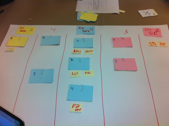
Here is a photo taken by team B:

We were able to finish the activity, but unfortunately, we did run short of time and could not analyze the results. I did promise this blog post for the attendees to share a few notes, photos and the Cumulative Flow diagram of each team.

At the end of the activity, I had the following data points:

• Team A completed 10 Stories
• Teams B and C had similar results: both finished 11 Stories
• Team D seemed like the less chaotic team, and did the highest number of stories: 12 Stories

On subsequent blog entries, I will share the feedback from the session (thanks!), upload activity photos, and the Cumulative Flow Diagram created by each team. If you were at the session and have either photos or the excel file, please send it over.

Here is the feedback I collected from this workshop.